📚 BOOK → ML Engineering (S. Bekman, 2026)
Rating: 10/10 | Intermediate to Advanced AI Engineers | Today's word: Halloween · ハロウィン · ליל כל הקדושים
🎵 "Somewhere, something incredible is waiting to be known." — Carl Sagan

Happy Monday, my dear anon friend.
This weekend, I had the chance to check out another very good (and delightfully opinionated) open-source book: Stas Bekman's Machine Learning Engineering. He is really smart, and I learned a lot from this book. His explanations of the details and advanced techniques involved in setting up hardware pipelines for training and inference are remarkably thorough and well-written. I must confess, though, that a good part of it was a bit advanced for my current level of knowledge. Still, it was worth reading for the general exposure (plus, I learned more about SLURM!), and I definitely intend to revisit this text later on.
As I read through the material, below are my highlights — with a moderate attempt at coherence — for my personal inventory (and perhaps as a way to connect with other friendly AI scientists and builders out there who love talking about the same things). As always, please remember our rules:
🤖 If you see a 👾, it means I found something particularly cool or learned something new.
🤖 If these notes look cool to you, it's your ✦moral duty✦ to read the original resources.
🤖 Just another blog, but not your usual blog: they're living notes that I change as I fancy.
🎃 INITIAL INSIGHTS
What do we want for Inference?
- Fast latency (users are used to msec response times and will leave if the response takes seconds)
- Fast throughput (how many concurrent queries can be processed)
- How much $$ is being spent per user (can we rent more GPUs to acquire more users and/or improve (1) and (2)?)
What are the workhorses of ML?
- An accelerator or a processing unit is what does most of the work.
- ML does a lot of parallel processing (SIMD) GPUs were used at the beginning, but now you additionally have TPUs, FPGAs, HPUs, QPUs, RDUs, etc. Recent CPUs are becoming used as accelerators as well, especially for inference.
Accelerators that can be used for training, finetuning and inferencing
Widely available:
- NVIDIA H200, B200, B300 - B300 systems are shipping.
- AMD MI325X, MI350X and MI355X - neoclouds primarily, but large CSPs have started offering AMD too.
- Intel Gaudi3 - on Intel’s cloud and via OEM servers.
Available, but locks you in:
- Google TPUs - fast, but a lock-in to one vendor and one cloud, and the software path is XLA rather than CUDA. It appears Google started to sell TPUs to some companies (outside of their cloud) - not officially confirmed, but it would weaken the lock-in argument if it holds.
- AWS Trainium2 - on AWS, also XLA.
- Cerebras WaferScale Engine - on Cerebras’ cloud.
Not yet available:
- NVIDIA Rubin - specs published but still marked preliminary.
- AMD MI455X - Helios volume deployments expected 2H-2026.
- SambaNova SN50 - shipping "in the second half of 2026"; SN40L is the current part.
- Intel Crescent Island - inference GPU, customer sampling announced for H2-2026; no published TFLOPS.
Regional:
- Huawei Ascend - real scale, but China-only in practice, and the specs are only on Huawei’s Chinese pages.
Accelerator Interoperability
In general most accelerators are supported by major frameworks like PyTorch or TensorFlow and the same code should run everywhere with small modifications as long as it doesn’t use any accelerator-specific functionality. For example, if your PyTorch application calls torch.mm - it should work everywhere, but if it includes custom CUDA kernels it’ll only work on NVIDIA GPUs and may be on the recent AMD MI-series.
- NVIDIA GPUs: all based on CUDA, which most training frameworks support. You can easily move between different NVIDIA GPUs and most things would work the same.
- AMD MI250/MI3xx: with PyTorch using ROCm you can run most CUDA-based software as is. This is really the only inter-operable accelerator with the NVIDIA stack.
- Intel Gaudi2/Gaudi3: if you use HF Transformers/Diffusers you can use optimum-habana. Trainer with NVIDIA GPUs it should be relatively easy to switch to train/infer on Gaudi2.
- Google TPU and AWS Trainium: both via XLA - PyTorch works, custom CUDA kernels don’t.
- Huawei Ascend: via CANN, with MindSpore first-party and PyTorch adaptation alongside it.
- Cerebras: is also working on PyTorch support via Cerebras Software Platform (CSoft) via XLA.
Also, in general, most ML code could be compiled into cross-platform formats like Open Neural Network Exchange (ONNX) which can be run on a variety of accelerators. This approach is typically used more often for inference workloads.
🎃 HARDWARE
Accelerators
- There exist two main ML workloads - training and inference. There is also the finetuning workload which is usually the same as training, unless a much lighter LORA-style finetuning is performed. The latter requires significantly fewer resources and time than normal finetuning.
- In language models during inference the generation is performed in a sequence - one token at a time. So it has to repeat the same forward call thousands of times one smallish
matmul(matrix multiplication or GEMM) at a time. And this can be done on either an accelerator, like GPU, or some of the most recent CPUs, that can handle inference quite efficiently. During training the whole sequence length is processed in one hugematmuloperation. So if the sequence length is 4k long, the training of the same model will require a compute unit that can handle 4k times more operations than inference and do it fast. Accelerators excel at this task. In fact the larger the matrices they have to multiply, the more efficient the compute.
- The other computational difference is that while both training and inference have to perform the same total amount of
matmulsin the forward pass, in the backward pass, which is only done for training, an additional 2x times ofmatmulsis done to calculate the gradients with regards to inputs and weights. And an additional forward is performed if activations recomputation is used. Therefore the training process requires at 3-4x morematmulsthan inference.
GPUs
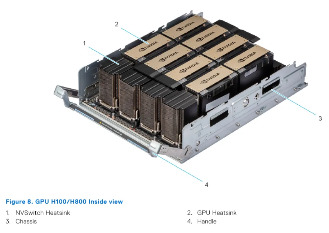
- As of today, ML clouds/HPCs already have B200s/B300s, and GB200/GB300 NVL72 racks are shipping. Rubin is expected to emerge in H2-2026.
- AMD’s MI325X is now widely available on Tier 2 cloud providers. MI355X is starting to emerge. MI455X hopefully in 2026. New: large CSPs started to offer AMD GPUs.
- Intel’s Crescent Island is an inference-oriented Xe3P data-center GPU, with customer sampling in H2-2026. Intel has not published TFLOPS.
HPU
- Intel’s Gaudi2 and Gaudi3 are available at Intel’s cloud.
- Falcon Shores project has been canceled.
TPU
- Google’s TPUs are available but they aren’t the most desirable accelerators because you can only rent them, and the software isn’t quite easily convertible between GPUs and TPUs, and so many (most?) developers remain in the GPU land, since they don’t want to be locked into a hardware which is a Google monopoly.
- Amazon’s Trainium2 is very similar to the TPU architecture and is available on AWS.
On Pods and racks
- Cerebras’ WaferScale Engine (WSE)
- SambaNova’s SambaRack (SN40L today, SN50 from H2-2026)
- dozens of different pod and rack configs that compose the aforementioned GPUs with super-fast interconnects.
Glossary
➡️ BLAS: Basic Linear Algebra Subprograms
➡️ CPU: Central Processing Unit
➡️ CTS: Custom Thermal Solution - a vendor-supported cooling option that allows a higher power limit than the default
➡️ CU: Compute Unit - AMD’s counterpart to NVIDIA’s SM
➡️ CUDA: Compute Unified Device Architecture - NVIDIA’s GPU programming platform
➡️ DCORE: the die core Intel reports Gaudi3 cache against; a Gaudi3 has 4 of them
➡️ DGX: NVIDIA’s turn-key accelerator server line
➡️ ECC: Error Correcting Code
➡️ FMA: Fused Multiply Add
➡️ FPGA: Field Programmable Gate Arrays
➡️ GA: Generally Available - the product can actually be bought or rented, as opposed to announced, sampling, or spec’d only
➡️ GCD: Graphics Compute Die
➡️ GEMM: General Matrix Multiply
➡️ GPU: Graphics Processing Unit
➡️ HBM: High Bandwidth Memory
➡️ HFU: Hardware FLOPS Utilization
➡️ HGX: NVIDIA’s accelerator baseboard that OEMs build their own servers around
➡️ HPC: High-performance Computing
➡️ HPU: Habana Gaudi AI Processor Unit
➡️ LLC: Last Level Cache
➡️ MAMF: Maximum Achievable Matmul FLOPS
➡️ MFU: Model FLOPS Utilization
➡️ MIG: Multi-Instance GPU - NVIDIA’s partitioning of one GPU into isolated instances
➡️ MME: Matrix Multiplication Engine
➡️ MSMF: Maximum Sustainable Matmul FLOPS
➡️ NVL72: an NVLink domain of 72 accelerators; likewise NVL8 and NVL36
➡️ OAM: OCP Accelerator Module - the Open Compute Project’s accelerator form factor
➡️ PSU: Power Supply Unit
➡️ PTX: Parallel Thread Execution - NVIDIA’s intermediate GPU instruction set
➡️ QPU: Quantum Processing Unit
➡️ RDU: Reconfigurable Dataflow Unit
➡️ SM: Streaming Multiprocessor - NVIDIA’s counterpart to AMD’s CU
➡️ SRAM: Static Random Access Memory\
➡️ TBP: Typical Board Power or Total Board Power, depending on vendor
➡️ TDP: Thermal Design Power or Thermal Design Parameter
➡️ TGP: Total Graphics Power
➡️ TPC: Tensor Processing Core
➡️ TPU: Tensor Processing Unit
➡️ WSE: Wafer Scale Engine - Cerebras’ whole-wafer accelerator
➡️ XCD: Accelerator Complex Die - AMD’s per-die cache reporting scope
➡️ XLA: Accelerated Linear Algebra - the compiler behind PyTorch/JAX on TPUs and Trainium
Metrics
The two metrics for a high ROI for ML training are:
- the speed at which the training will finish, because if the training takes 2-3x longer than planned, your model could become irrelevant before it was released - time is everything in the current super-competitive ML market.
- the total $$ spent to train the model, because if the training takes 2-3x longer than planned, you will end up spending 2-3x times more.
- The most critical component is network, then storage, and the least critical ones are CPU and CPU memory (at least for a typical training workload where any CPU limitations are compensated with multiple DataLoader workers).
- The term TFLOPS defines how many trillions of
FloatingPointOperationsthe chip can perform in a second. The more the better. There is a different definition for different data types.
- The term FLOPS could mean either the total number of
FloatingPointOperations, e.g. when counting how many FLOPS a single Transformer iteration takes, and it could also meanFloatingPointOperationsper second - so watch out for the context. When you read an accelerator spec it’s almost always a per second definition. When model architectures are discussed it’s usually just the total number ofFloatingPointOperations.
Theoretical FLOPS = compute_unit_clock_speed * FLOPs_per_clock_cycle_per_compute_unit * num_compute_units

where:

compute_unit_clock_speed - how many times the compute unit clock ticks per second in Hz
flops_per_clock_cycle_per_compute_unit - the number of floating point operations the compute unit can execute per clock cycle
num_compute_units - how many units there are in the device FLOPs per clock cycle per compute unit is usually not published, but what one often finds is the FMAs per clock cycle per compute unit specs
- The problem with the advertised theoretical peak FLOPS is that they are very theoretical and can’t be achieved in practice even if all the perfect conditions have been provided. Each accelerator has its own realistic FLOPS which is not advertised and there are anecdotal community reports that do their best to find the actual best value.
- MAMF stands for Maximum Achievable Matmul FLOPS, which is a term coined by yours truly, and MSMF for Maximum Sustainable Matmul FLOPS - what the accelerator holds once it is saturated at its power limit. Both are very practical for those who do performance optimization work.
- The accelerators use High Bandwidth Memory (HBM) which is a 3D version of SDRAM memory. For example, the 80GiB A100-SXM comes with HBM2e at 2.0TBps, and the 80GiB H100-SXM comes with HBM3 at 3.35TB.
Peak Bandwidth
bandwidth (bytes/sec) = memory clock (Hz) * bus width (bytes) * 2
- The
*2is because HBM, like all Double Data Rate memory, transfers on both the rising and the falling clock edge - hence one transfer per half-cycle rather than per cycle. - The bus width is the whole memory interface summed across every stack, not one stack’s width, which is the easiest of the three to get wrong.
Memory Clock
import torch

p = torch.cuda.get_device_properties(0)

# memory_clock_rate is the *peak* clock in kHz; memory_bus_width is in bits
bw = p.memory_clock_rate * 1e3 * (p.memory_bus_width / 8) * 2 / 1e12

print(f"{p.name}: {p.memory_clock_rate/1e6:.3f}GHz x {p.memory_bus_width}-bit bus → {bw:.2f}TBps")
- Two things to watch. Take the peak memory clock rather than the current one - an idle accelerator clocks its memory down, so nvidia-smi’s Clocks section will read low while Max Clocks reads the figure this arithmetic needs, and PyTorch’s
memory_clock_rateis already the peak. And this gives the theoretical ceiling; what a real workload achieves is lower, which is what Maximum Achievable Matmul FLOPS is to TFLOPS.
- High performance cache is used for storing frequently used instructions and data. L1 is usually the smallest and fastest, then L2 is a bit larger and a bit slower and there can be an L3 cache which is even bigger and slower. All these caches massively reduce trips to HBM.
- Clock speed, also known as clock rate this spec tells us at which frequency the card runs. As hardware becomes faster newer generations will typically increase the clock speed.
- Clock frequency is useful for calculating theoretical TFLOPS within an architecture, but raw MHz alone does not rank performance across different architectures.
- NVIDIA defines TGP as the total electrical power for the GPU core, onboard memory, and supporting board circuitry. Its DGX B200 power controls separately expose a 1000W maximum TGP, a 700W default set point, the configured set point, and current measured power.
- AMD lists MI250X with 500W TDP and 560W peak TBP, so for this OAM module the published peak TBP is 60W above its TDP.
- Kernel time is not a function of tensor shapes alone. The values flowing through a GEMM change how hard the chip works, and that feeds back into the clock.
- Dynamic power is roughly proportional to clock frequency times the number of transistors that flip. High-entropy or "unpredictable" bit patterns flip more transistors per cycle than sparse, sorted, or all-zero patterns, so the same-shape matmul draws more power.
- Model FLOPS Utilization (MFU) metric measures TFLOPS achieved against theoretical TFLOPS. Usually when one scores around 50% MFU it’s considered a win. But this gives us no indication how far are we from the real achievable throughput.
- MAMF (Maximum Achievable Matmul FLOPS) is the rate a short burst reaches at the boost clock. Each shape gets 10 bursts of 20 back-to-back iterations, and each burst starts after 0.25s of idle so the SM clock climbs back to boost.
- MSMF (Maximum Sustainable Matmul FLOPS) is the highest rate a shape holds without falling, over a timed window on a GPU that has run at full load long enough for its clock to settle.
What CPU memory is needed for in ML workloads
- Loading the model weights, unless they are loaded directly onto the GPUs - this is usually a transitory memory usage that goes back to zero once the model has been moved to GPUs.
- Saving the model weights. In some situations each GPU writes its own checkpoint directly to the disk, in other cases the model is recomposed on the CPU before it’s written to disk - this too is a transitory memory usage.
- Possible parameter and optimizer state offloading when using frameworks like DeepSpeed. In which case quite a lot of CPU memory might be needed.
- Activations calculated in the forward pass, and which need to be available for the backward path can also be offloaded to CPU, rather than discarded and then recomputed during the backward pass to save the unnecessary overhead.
DataLoaderis usually one of the main users of CPU memory and at times it may consume very large amounts of memory. Typically there are at least 2x 8 DL workers running on each node, so you need enough memory to support at least 16 processes each holding some data.
- The software itself and its dependent libraries uses a bit of CPU memory, but this amount is usually negligible.
IO
Synchronous vs asynchronous IO
- In synchronous IO the client submits an IO request and wait for it to be finished before start the next request.
- In asynchronous IO the client may submit multiple IO requests one after another without waiting for any to finish first. This requires that the target device can queue up multiple IO requests.
Sequential vs Random access IO
- Sequential access IO is when you read blocks of data one by one sequentially (think a movie). Examples: reading or writing a model’s checkpoint file all at once, loading a python program, and installing a package.
- Random access IO is when you’re accessing part of a file at random. Examples: database querying, reading samples from a pre-processed dataset in a random fashion, and moving around a file using seek.
IO Metrics
The three main storage IO metrics one typically cares about are:
- Throughput or Bandwidth (bytes per second - can be MBps, GBps, etc.)
- IOPS (Input/output operations per second that a system can perform) - IOPS measures how many input and/or output operations a given storage device or a cluster can perform per second. Typically read and write IOPS won’t be the same. And for many systems it’ll also depend on whether the operation is sequential or random.
- Latency (msecs or usecs)
So a storage system will have 4 different IOPS rates:
- IOPS of random reads
- IOPS of random writes
- IOPS of sequential reads
- IOPS of sequential writes
Inter-Node and Intra-Node Networking Hardware
Cluster networks
Each node of the cluster has 3 networks, each running at a very different speed from each other:
- Frontend
- Backend
- Out-of-band
Frontend networking
- Frontend networking is typically for the Internet connection (e.g. downloading python packages and offloading to the cloud storage), distributed network storage (e.g. checkpoints and datasets) and orchestration (e.g. SLURM and Kubernetes).
- As of 2026-08 a typical node is likely to have a single 100-400Gbps connection.
Backend networking
- Backend networking is to perform GPU-to-GPU connectivity which allows training and inference to scale to multiple accelerators (e.g. all-reduce, all-gather and other collective comms).
- This is the most important part of the AI cluster.
Out-Of-Band networking
- Out-Of-Band (OOB) networking is used for bootstrapping backend networking, monitoring node’s health, remote re-imaging of the nodes, etc.
- It typically uses a single slow 1Gbps ethernet connection.
RDMA networking
- Remote Direct Memory Access is like DMA (Direct Memory Access) on the node, but across nodes.
- It allows data exchange between nodes w/o the overhead using the local processor, OS kernel and caches, which is what TCP/IP uses.
- The 3 main implementations are:
- InfiniBand
- RDMA over Converged Ethernet (RoCE) (IB or UDP-based RDMA)
- iWARP (TCP-based RDMA)
Intra-node networking
- This is also known as scale-up networking.
- There are multiple platforms/solutions out there that provide intra-node networking:
- Generic: PCIe
- NVIDIA: NVLink and NVSwitch
- AMD: Infinity Fabric
- Intel: Gaudi2, Gaudi3
- AWS: NeuronLink (Trainium)
- Google: ICI (TPU)
- Huawei: UB Link (Ascend)
Inter-node networking
- This is also known as scale-out networking.
- As inter-node hardware used to be about of an order of magnitude slower than intra-node hardware in this universe Gbps are used instead of GBps. (1GBps = 8Gbps) (The links themselves are still about an order of magnitude apart, but the practical gap for collectives is much smaller, because an inter-node collective also does most of its work over the intra-node).
- When it comes to inter-node networking hardware, there are the well established InfiniBand from NVIDIA and a few other players, various NVLink-based NVIDIA products and there are many new comers that mainly are coming from compute cloud providers who can’t compete on the slim margin renting out someone else’s hardware so they build their own (AWS EFA, GCP GPUDirect-TCPX), and there are also HPE and Cornelis Networks with recently updated products.
- Typically the more "hops" the message has to travel, the bigger the latency. 2 accelerators residing on the same node and connected directly to each other (e.g., NVLink) will have the least amount of latency. If their communication path traverses a PCIe switch the latency will be bigger. 2 accelerators residing on 2 different nodes sharing a single switch will have a bigger latency because there is a switch to traverse. The further they get away from each other, the more switches the message has to travel through, the bigger the latency.
Algorithms
The collective communications may have a variety of different implementations, and comm libraries like nccl may switch between different algorithms depending on internal heuristics, unless overridden by users:
- Ring
- Tree
🎃 ORCHESTRATION
- There are many container/accelerator orchestration solutions - many of which are open source.
SLURM
- Simple Linux Utility for Resource Management, which you’re guaranteed to find on most HPC environments and typically it’s supported by most cloud providers. It has been around for more than 2 decades.
- SLURM builds on top of Unix and so it just makes multi-node coordination easier.
These are frameworks allowing you to run SLURM on top of Kubernetes:
- Slinky - a framework from the creators of SLURM
- Soperator - from Nebius
- CoreWeave never released their SUNK open source, so it’s only available to its customers
Kubernetes
- Open source system for automating deployment, scaling, and management of containerized applications.
- In general IMHO kubernetes is the wrong environment for doing training work, with SLURM being a much more user-friendly orchestration.
Others
- dstack is a lightweight, open-source alternative to Kubernetes & SLURM, simplifying AI container orchestration with multi-cloud & on-prem support. It natively supports NVIDIA, AMD, & TPU.
- SkyPilot is a framework for running AI and batch workloads on any infra, offering unified execution, high cost savings, and high GPU availability.
- OpenHPC provides a variety of common, pre-built ingredients required to deploy and manage an HPC Linux cluster including provisioning tools, resource management, I/O clients, runtimes, development tools, containers, and a variety of scientific libraries.
- run.ai - got acquired by NVIDIA and is planned to be open sourced soon.
- Docker Swarm is a container orchestration tool.
- IBM Platform Load Sharing Facility (LSF) Suites is a workload management platform and job scheduler for distributed high performance computing (HPC).
🎃 TRAINING
Glossary
➡️ BS: Batch Size - here we mean batch size per GPU; often, it is also referred to as MBS (micro-batch size)
➡️ GAS: Gradient Accumulation Steps - how many forward/backward cycles to perform before one full iteration is complete
➡️ GBS: Global Batch Size - total batch size per iteration; may include gradient accumulation
➡️ PP: Pipeline Parallelism
➡️ TFLOPS: Trillion FLOPs per second – FLOP
Model Parallelism
In the modern Machine Learning the various approaches to parallelism are used to:
- Overcome GPU memory limitations.
- Significantly speed up training - finish training that would take a year in hours
- Two main approaches are used to enable training and inferring models that are bigger than the accelerator’s memory:
- 3D parallelism - very network efficient, but can be very invasive into the modeling code and require a lot more work to make it work correctly.
- ZeRO parallelism - not very network efficient, but requires close to zero changes to the modeling code and very easy to make to work.
Scalability concepts
- Data Parallelism (DP) - the same setup is replicated multiple times, and each being fed a slice of the data. The processing is done in parallel and all setups are synchronized at the end of each training step.
- TensorParallelism (TP) - each tensor is split up into multiple chunks, so instead of having the whole tensor reside on a single GPU, each shard of the tensor resides on its designated GPU. During forward and backward processing the shards execute concurrently and exchange partial activations or gradients at layer-specific boundaries, often using all-reduce, all-gather, or reduce-scatter rather than synchronizing only at the end of the step. This is what one may call horizontal parallelism, as the splitting happens on horizontal level.
- PipelineParallelism (PP) - the model is split up vertically (layer-level) across multiple GPUs, so that only one or several layers of the model are places on a single GPU. Each GPU processes in parallel different stages of the pipeline and working on a small chunk of the batch.
- Zero Redundancy Optimizer (ZeRO) - Also performs sharding of the tensors somewhat similar to TP, except the whole tensor gets reconstructed in time for a forward or backward computation, therefore the model doesn’t need to be modified. It also supports various offloading techniques to compensate for limited GPU memory. Sharded DDP is another name for the foundational ZeRO concept as used by various other implementations of ZeRO.
- Sequence Parallelism - training on long input sequences requires huge amounts of GPU memory. This technique splits the processing of a single sequence across multiple GPUs.
- Expert Parallelism - Mixture-Of-Experts (MoE) can be partitioned so that each expert has a dedicated GPU (or several of them).
Data Parallelism
- ZeRO-powered data parallelism (ZeRO-DP): it can be difficult to wrap one’s head around it, but in reality the concept is quite simple. This is just the usual DataParallel (DP), except, instead of replicating the full model params, gradients and optimizer states, each GPU stores only a slice of it. And then at run-time when the full layer params are needed just for the given layer, all GPUs synchronize to give each other parts that they miss - this is it.
Tensor Parallelism
- In Tensor Parallelism each GPU processes only a slice of a tensor and only aggregates the full tensor for operations that require the whole thing.
- The main building block of any transformer is a fully connected
nn.Linearfollowed by a nonlinear activation GeLU.
- Following the Megatron’s paper notation, we can write the dot-product part of it as
Y = GeLU(XA), whereXandYare the input and output vectors, andAis the weight matrix.
Sequence Parallelism
- ML tasks, such as DNA sequencing, may require training with very long sequence lengths (e.g. 256K), and even normal LLMs could be trained on sequences of 10k and longer.
- Self-Attention, which is a key component of Transformers, has quadratic compute complexity with respect to sequence length for standard dense attention. Kernels that materialize the full sequence-by-sequence attention matrix also require quadratic temporary memory. Memory-efficient kernels such as
FlashAttentionavoid storing that matrix and keep attention memory linear in sequence length without removing the quadratic compute.
- At sufficiently long sequence lengths, even a batch size of 1 may not fit on a single GPU, so sequence parallelism partitions work along the sequence dimension. This increases the supported sequence length, but does not make it unlimited: the practical limit still depends on aggregate accelerator memory, compute time, communication overhead, and kernel constraints.
- As this type of parallelism is orthogonal to the other parallelization types described in this document, it can be combined with any of them, leading to 4D, ZeRO-DP+SP and other combinations.
Expert Parallelism
- When Mixture-Of-Experts (MoE) is used (in particular during inference) one could give each expert its own accelerator (or a few if one isn’t enough), which is referred to as Expert Parallelism (EP).
- This adds another dimension for parallelization and can significantly speed things up for large batches that are likely to hit all of the experts.
- Instead of communicating model weights, in EP tokens are being communicated instead. EP leads to a more efficient compute as matrix multiplication then deal with bigger inputs.
Anatomy of Model’s Operations
Transformers architecture includes 3 main groups of operations grouped below by compute-intensity:
1️⃣ Tensor Contractions
Linear layers and components of Multi-Head Attention all do batched matrix-matrix multiplications. These operations are the most compute-intensive part of training a transformer.
2️⃣ Statistical Normalizations
Softmax and layer normalization are less compute-intensive than tensor contractions, and involve one or more reduction operators, the result of which is then applied via a map.
3️⃣ Element-wise Operators
These are the remaining operators: biases, dropout, activations, and residual connections. These are the least compute-intensive operations.
Memory
The components on GPU memory are:
- model weights
- optimizer states
- gradients
- forward activations saved for gradient computation
- temporary buffers
- functionality-specific memory
A typical model trained in mixed precision with AdamW requires 18 bytes per model parameter plus activation memory and temp memory.
Model Weights
- 4 bytes * number of parameters for
fp32training - 6 bytes * number of parameters for mixed precision training (maintains a model in
fp32and one infp16/ bf16in memory)
Optimizer States
- 8 bytes * number of parameters for normal AdamW (maintains 2 states)
- 4 bytes * number of parameters for AdamW running at
bf16. See this work that uses AnyPrecisionAdamW. - 4 bytes * number of parameters for optimizers like SGD with momentum (maintains only 1 state) or LION, or Adafactor (and others) (Adafactor uses some additional memory beside 4 bytes)
- 2 bytes * number of parameters for 8-bit AdamW optimizers like bitsandbytes
Gradients
- 4 bytes * number of parameters for either
fp32precision and in some frameworks with mixed half-precision training. - 2 bytes * number of parameters for non-mixed half-precision and in some frameworks with mixed half-precision training.
Forward activations
A rough breakdown of activation memory per GPU:
- Activation working memory:
dtype_size x num_of_hidden_states_copies x bs x seqlen x hidden_size - Activation checkpoints memory:
dtype_size x num_layers x bs x seqlen x hidden_size - Logits working memory:
fp32_size x bs x seqlen x vocab_size
Where:
dtype_size: size of the one element of dtype being used, e.g. 1 byte forfp8, 2 forbf16, 4 forfp32, etc.fp32_size: 4 bytesbs: batch sizehidden_size: hidden size of the modelseqlen: the sequence lengthnum_layers: the number of layers the model hasvocab_size: vocabulary sizedtype_size x bs x seqlen x hidden_sizeis the size of thehidden_statestensor.
Memory fragmentation
- As the model allocates and frees tensors, the GPU memory could fragment. That is there could be enough free memory to allocate, say, 1GiB of contiguous memory, but it could be available in 100s of small segments spread out through the memory and thus even though the memory is available it can’t be used unless very small allocations are made.
- Environment variable
PYTORCH_ALLOC_CONFcomes to help and allows you to replace the default memory allocation mechanisms with more efficient ones. For more information see Memory management.
Batch sizes
- micro batch size (MBS), also known as batch size per GPU - this is how many samples a single GPU consumes during a model’s single forward call.
- global batch size (GBS) - this is the total amount of samples consumed between two optimizer steps across all participating GPUs.
Model replica
- How many GPUs are needed to fit the full model.
- If the model fits into a single GPU a model replica takes 1 GPU. Usually then one can use multiple GPUs to perform Data Parallelism.
- If the model doesn’t fit into a single GPU, it’d usually require some sort of sharding technique - it can be Tensor Parallelism (TP), Pipeline Parallelism (PP), or ZeRO Data Parallelism (ZeRO-DP).
- You can have as many data streams as there are replicas. Which is the same as the value of DP.
Gradient Accumulation
- The idea behind gradient accumulation is to instead of calculating the gradients for the whole batch at once to do it in smaller steps. The way we do that is to calculate the gradients iteratively in smaller batches by doing a forward and backward pass through the model and accumulating the gradients in the process.
- When enough gradients are accumulated we run the model’s optimization step. This way we can easily increase the overall batch size to numbers that would never fit into the GPU’s memory. In turn, however, the added forward and backward passes can slow down the training a bit. Gradient Accumulation Steps (GAS) is the definition of how many steps are done w/o updating the model weights.
Gradient Checkpointing
- Enabling gradient checkpointing allows one to trade training throughput for accelerator memory. When this feature is activated instead of remembering the outputs of, say, transformer blocks until the backward pass is done, these outputs are dropped. This frees up huge amounts of accelerator memory. But, of course, a backward pass is not possible without having the outputs of forward pass, and thus they have to be recalculated.
- This, of course, can vary from model to model, but typically one pays with about 20-25% decrease in throughput, but since a huge amount of GPU memory is liberated, one can now increase the batch size per GPU and thus overall improve the effective throughput of the system. In some cases this allows you to double or quadruple the batch size if you were already able to do a small batch size w/o OOM. (Recent papers report as high as 30-40% additional overhead.)
Memory-efficient optimizers
- The most common optimizer is Adam. It and its derivatives all use 8 bytes per param (2x fp32 tensors - one for each momentum), which account for almost half the memory allocation for the model, optimizer and gradients. So at times using other optimizers may save the day, if they successfully train that is. Not all optimizers are suitable for all training tasks.
- 4-byte optimizers: There are optimizers like Adafactor that need only 4 bytes. Same goes for the LION optimizer.
- 2-byte optimizers: There are quantized solutions like
bnb.optim.Adam8bitwhich uses only 2 bytes instead of 8 (1 byte per momentum).
NUMA affinity
- Non-uniform memory access (NUMA) is a computer memory design used in multiprocessing, where the memory access time depends on the memory location relative to the processor.
- As modern servers have more than one CPU to get the best performance accelerators residing in the same NUMA node as the corresponding CPU should have the processes bound to that same NUMA node.
Fault Tolerance
- Regardless of whether you own the ML training hardware or renting it by the hour, in this ever speeding up domain of ML, finishing the training in a timely matter is important. As such if while you were asleep one of the GPUs failed or the checkpoint storage run out of space which led to your training crashing, you’d have discovered upon waking that many training hours were lost.
- Due the prohibitively high cost of ML hardware, it’d be very difficult to provide redundancy fail-over solutions as it’s done in Web-services. Nevertheless making your training fault-tolerant is achievable with just a few simple recipes.
- Always plan to have more nodes than needed.
Reproducibility and Determinism
- When debugging always set a fixed seed for all the used Random Number Generators (RNG) so that you get the same data/ code path on each re-run.
- On GPU, seeding alone isn’t enough for bitwise-reproducible results: cuDNN and cuBLAS are free to pick different (but individually valid) algorithms from run to run for the same op, so a truly deterministic re-run also requires forcing them to always pick the same, deterministic ones - that’s what the
cudnn.benchmark,use_deterministic_algorithms()andCUBLAS_WORKSPACE_CONFIGsettings take care of.
Selecting Training Hyper-Parameters And Model
Tensor Precision / Data Types
Floating point formats:
• fp32 - 32 bits
• tf32 - 19 bits (NVIDIA Ampere+)
• fp16 - 16 bits
• bf16 - 16 bits
• fp8 - 8 bits (E4M3 and E5M2 formats)
• fp6 - 6 bits
• fp4 - 4 bits
The new formats that are being adopted by new hardware are:
• fp4: float4_e2m1fn
• fp6: float6_e2m3fn and float6_e3m2fn
• fp8: float8_e3m4, float8_e4m3, float8_e4m3b11fnuz, float8_e4m3fn, float8_e4m3fnuz, float8_e5m2, float8_e5m2fnuz, float8_e8m0fnu
Integer formats used in quantization:
• int8 - 8 bits
• int4 - 4 bits
• int1 – 1 bit
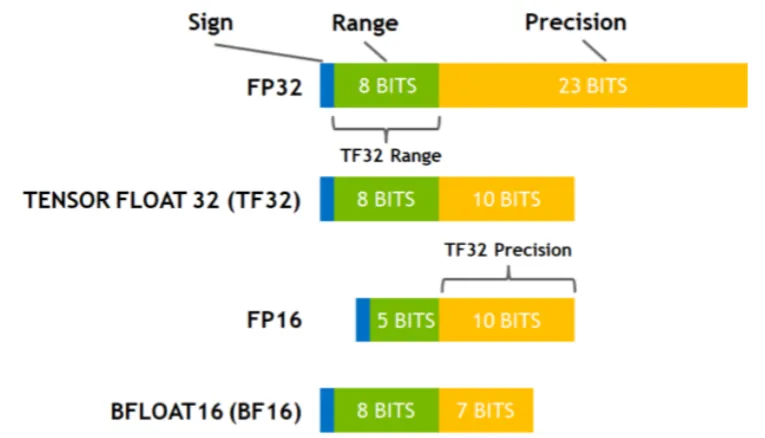
ML dtype progression
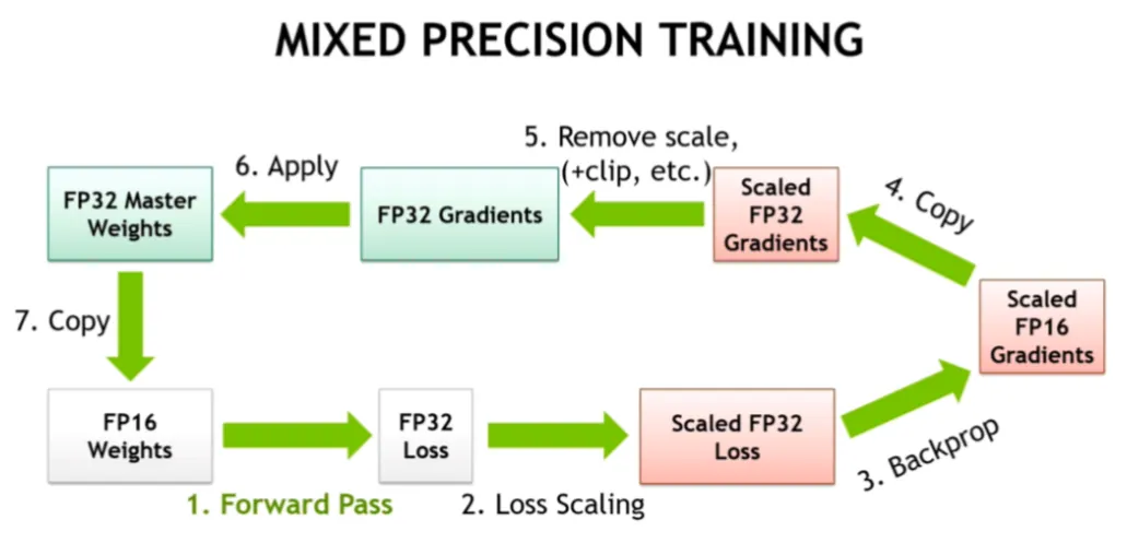
- Originally ML was using
fp32, but it was very slow. - Next mixed-precision was invented using a combination of
fp16andfp32, which tremendously sped up the training speed. fp16proved to be not very stable and training LLM was extremely difficult. Luckilybf16came out and replacedfp16using the same mixed precision protocol. This made the LLM training much more stable.- Then
fp8came and mixed precision could switch to that, which makes the training even faster.
FP4 formats
- An
fp4element has 16 bit patterns: ±0, ±0.5, ±1, ±1.5, ±2, ±3, ±4 and ±6. - That is far too few to cover a tensor’s range with one scale, so
fp4is only usable block-scaled: every small block of elements shares a scale that stretches those values over the block’s actual range. - There are two block-scaled
fp4formats, and they differ only in that scale. Sorted by block size, descending.
TF32
TF32is a magical datatype that is available on NVIDIA GPUs since Ampere, and which allowsfp32matmulsperformed at a much faster speed than normalfp32matmulswith a small precision loss.
When to use fp32 accumulators
- Whenever a low-precision dtype is used one has to be careful not to accumulate intermediary results in that dtype.
- LayerNorm-like operations must not do their work in half-precision, or they may lose a lot of data. Therefore when these operations are implemented correctly they do efficient internal work in the dtype of the inputs, but using the
fp32accumulation registers and then their outputs are downcast to the precision of the inputs.
Emulating multiple GPUs with a single GPU
- With NVIDIA A100 you can use MIG to emulate up to 7 instances of GPUs on just one real GPU, but for years you couldn’t use those instances for anything but standalone use - e.g. you couldn’t do DDP or any NCCL comms over those GPUs.
- NCCL 2.31 (2026) added experimental support for communicators that span MIG instances, so a single physical GPU can now stand in for a small multi-GPU node and you can run DDP, FSDP, ZeRO and any NCCL collective across its instances.
- Traffic between MIG instances never leaves the GPU - NCCL logs every channel as P2P/CUMEM with no socket or PCIe fallback anywhere in the run - so the limit is the memory bandwidth the instance owns, which is set by its memory slices and barely at all by its Sms.
- Until NVIDIA overcomes the odd 7-instance per GPU limit, if you want to do a 3D parallelism, you need at least 8 GPUs or instances. So for a time being we have to use 2 GPUs to get to 8.
- Keep an emulated multi-GPU job inside a single physical GPU. Crossing to a second GPU costs a factor of 10 against 4 instances on one GPU (26.8 against 273.8GBps at 512MiB), and leaves you at 5% of what 8 real GPUs do. Though if you’re working with a tiny model and payload it probably doesn’t matter much for dev purposes.
- Do keep in mind that this emulates the topology of a multi-GPU job and not its performance - each rank also gets only a fraction of the SMs and a fraction of the memory, so it’s a development and testing tool, not a way to measure throughput.
🎃 INFERENCE
Glossary
➡️ CLA: Cross-Layer Attention
➡️ FHE: Fully Homomorphic Encryption
➡️ GQA: Grouped-Query Attention
➡️ ITL: Inter-Token Latency
➡️ KV: Key-Value
➡️ LPU: Language Processing Unit™
➡️ MHA: Multi-Head Attention
➡️ MLA: Multi-Latent Attention
➡️ MPC: Secure Multi-Party Computation
➡️ MQA: Multi-Query Attention
➡️ PPML: Privacy-Preserving Machine Learning
➡️ QPS: Queries Per Second
➡️ TPOT: Time Per Output Token
➡️ TTFT: Time to First Token
Prefill and Decode
When doing inference there are 2 stages:
1️⃣ Prefill: the model processes the prompt tokens in parallel, similar to training, and builds the KV cache used during generation. Prefill is usually compute-bound. Its latency contributes directly to TTFT and generally increases with input length; long prompts or insufficient compute can make prefill a major part of request latency.
2️⃣ Decode: During ordinary autoregressive decoding, the model generates one output token at a time based on the prompt and previously generated tokens. This sequential dependency prevents parallelizing output-token steps within one sequence, and decode is often memory-bandwidth-bound. Which stage matters most depends on the workload and metric. TTFT is sensitive to prompt length, prefill efficiency, scheduling, and queueing; TPOT/ITL primarily characterizes decode; end-to-end latency depends on input length, output length, batching, load, and hardware.
Anatomy of Model’s Memory Usage
The inference memory usage is quite different from training. Here we have:
- Model weights
- KV cache - crucial to not need to recalculate past tokens for each new generated token
- Activation memory - this is the processing temporary memory which would depend on a batch size and a sequence length
Model Weights
Bytes per parameter for each dtype:
- 4 bytes * number of parameters for
fp32 - 2 bytes * number of parameters for
fp16/bf16 - 1 byte * number of parameters for
fp8/int8 - 0.75 bytes * number of parameters for
fp6or 6-bit quantization - 0.625 bytes * number of parameters for 5-bit quantization
- 0.5 bytes * number of parameters for
fp4/int4 - 0.375 bytes * number of parameters for 3-bit quantization
- 0.25 bytes * number of parameters for 2-bit quantization
- 0.125 bytes * number of parameters for 1-bit quantization
Example: Meta-Llama-3.1-8B in bf16 will need 2 (bf16 bytes) * 8B (num of params) = 16GB (approximately)
KV Caching
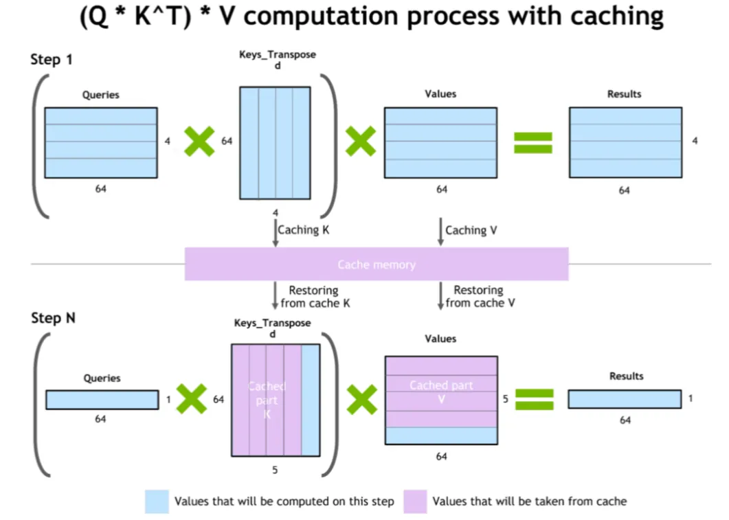
- It’d be very expensive to recalculate all the previous KV (Key Value) values before each new token is generated and thus they are cached in accelerator’s memory.
- Newly computed KV-values are appended to the existing cache.
- KV cache size is directly proportional to the input sequence length and batch size.
- Past query values aren’t used in the attention mechanism and thus don’t need to be cached.
- A KV cache of 1 token requires:
dtype_bytes * 2 * num_hidden_layers * hidden_size * num_key_value_heads / num_attention_heads bytes

where:

- dtype_bytes is bytes per dtype: 4 bytes for fp32, 2 bytes for bf16/fp16, etc.
- 2 stands for keys + values as there are 2 of them.
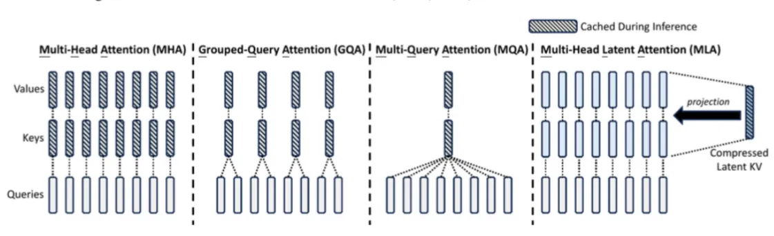
- num_key_value_heads / num_attention_heads is the factor that will depend on whether multi-query (MQA), grouped-query (GQA) or multi-head attention (MHA) is used
Examples:
- 1 token Meta-Llama-3.1-8B in bf16 will need:
2 (bf16 bytes) x 2 (keys+values) x 32 (num_hidden_layers) x 4096 (hidden_size) x 8 (num_key_value_heads) / 32 (num_attention_heads) / 10**6 = 0.131MB - This model uses GQA so it uses 1/4th of the vanilla MHA.
- A batch size of 1 of 1024 tokens will need
0.131*1024 = ~134MB. - A batch size of 128 of 1024 tokens each will need
0.131*1024*128 / 10**3 = ~17.2GB. - The KV cache for Meta-Llama-3.1-8B would have taken 4x more memory per token if it were to use MHA, 8x less memory if it were to use MQA.
- In this case the model has
num_key_value_heads=8andnum_attention_heads=32, hence MQA and GQA use 32x and 4x less memory than MHA, correspondingly. - DeepSeek v3 introduced Multi-Latent Attention (MLA) which compresses the Key and Value into a latent vector, which further reduces the KV-cache size.
SwiftKV
- SwiftKV was invented to deal with the common situation of 10:1 ratio of prefill vs decode use-cases, reducing inference computation during prompt processing rather than just compressing memory.
- By combining model rewiring and knowledge-preserving self-distillation, SwiftKV achieves substantial reductions in computational overhead during inference with minimal accuracy loss, leading to transformative improvements in throughput, latency and cost efficiency for enterprise LLM workloads by up to 2x.
Online vs Offline inference
- When you have users that send queries in real time - this is Online inference, also known as Deployment or Interactive inference. Examples: chatbot, search engines, general REST APIs. In this case one always runs an inference server and there could be various clients querying it.
- When you have a file with hundreds or thousands of prompts that you need to run inference on - this is Offline inference, also known as batch inference. Examples: benchmark evaluation and synthetic data generation. In this case the inference server is often not needed and the inference is run directly in the same program that sends the query (client and server in one application).
- The 2 main use cases are often optimized for different performance metrics - the online inference use case requires a very low TTFT and low latency, whereas the offline inference requires high throughput. The combined prefill and decode token processing throughput is the key metric for any type of inference because it defines the total cost of the inference service.
- In the case of online inference, the better the combined throughput the more users can be served with the same hardware.
- For offline inference, it’s clear that the faster the inference is done, the smaller the compute costs will be.
Batching
- Processing the decoding stage one token at a time is extremely accelerator-inefficient.
- Batching multiple queries together improved the accelerator utilization and enables processing multiple requests at once.
- The maximum possible batch size depends on how much memory is left after loading the model weights and filling the KV-cache with intermediate states.
Static batching
- This is the naive straightforward batching where the first N queries are batched together.
- The problem here is that if many queries have finished generating they will have to wait for the longest to generate query to complete before they can be returned to the caller - greatly increasing the latency.
Continuous Batching or In-flight batching
- Process where the generation engine removes completed results as soon as they are done and replacing them with new queries, without waiting for the whole batch to complete.
- So that a sequence in position 0 in the batch could be generating its 10th token, while a sequence in position 1 in the batch could be just starting its first token generation, and position 3 is producing its last token.
- This improves the response time, since a sequence that already finished can be returned immediately and there is no need for a new prompt to wait for the next batch to become available. Of course, if all of the compute is fully busy, and there are no new openings in the batch, then some requests will have to wait before the compute will start processing those.
Paged Attention
- Paged Attention is very popular with inference servers as it allows for a very efficient accelerator memory utilization, by the virtue of approaching the accelerator memory like the OS memory using paging, which allowed dynamic memory allocation and prevents memory fragmentation.
Decoding methods
- The main decoding methods are:
1️⃣ Greedy decoding: when the model always chooses the token with the highest probability. This is the fastest decoding method but it doesn’t always generate the best outcome, since it may choose a less ideal token path and miss out on a great
future sequence of tokens. One of the main issues with this method is creation of loops, where the same sentence is repeated again and again.
2️⃣ Beam search: overcomes the limitation of greedy decoding by generating multiple outputs at the same time, so instead of following the highest probability - with beam size of 3 it follows top 3 probabilities at each new token, then discards all but
the 3 sub-paths out of 9 (3*3), that lead to the highest total probability of all tokens in the chain. Then at the end the path with the highest probability of all tokens is chosen. This method is slower than greedy decoding because it has to generate n times more tokens and it requires n times more memory.
Sampling
- Sampling-based decoding introduces randomness.
- But, of course, choosing random words will not lead to a good result, so we still want greedy decoding like certainty but making it more interesting/alive by adding controlled randomness to it.
- The most common sampling methods are: Top-K (chooses the top k tokens based on their logit probability and then randomly picks one of those tokens) and Top-p (like Top-K Sampling, but the K varies for each next token and is calculated by adding up the top token probabilities till the threshold p is reached. So if there are predictions that the model is much more certain about only those will be considered).
Temperature
- Temperature is an independent logits transformation that can be combined with Top-K or Top-p sampling, both of them, or neither.
t = 0.0: literal softmax temperature division by zero is undefined. Some APIs use zero as shorthand for greedy decoding while others reject it, so use the API’s explicit greedy mode when available.0.0 < t <1.0: the probabilities are pushed further apart, so the closer to 0.0 the less randomness - somewhere between precise and balanced use cases.t = 1.0: has no impact on sampling - the original training distribution is preserved here - balanced relevance and diversity use cases.t > 1.0: the probabilities are pushed closer together, creating a lot more randomness - creative use cases.
- To really understand the impact, the temperature factor typically gets applied to the log probabilities just before or as part of the Softmax operation.
scaled_logits = logits / temperature
probs = softmax(scaled_logits)
- The softmax operation turns logit differences into probability ratios - when we divide by
t < 1.0, we make these differences larger, causing more extreme probability ratios and a more peaked distribution. - When we divide by
t > 1.0, we make these differences smaller, causing more similar probability ratios and a more uniform distribution. - As
tapproaches0from above, the highest logit dominates the distribution, but literal division by zero is avoided in practice. - For any positive temperature, scaling doesn’t change the logit rank order, so a pure greedy argmax chooses the same token. It still changes sampling probabilities.
- With Top-K, the same K candidates remain eligible but their relative sampling probabilities change.
- With Top-p, temperature can change both which tokens enter the nucleus and their relative probabilities.
- Beam-search behavior depends on the implementation and its sequence scoring, so it shouldn’t be assumed to be invariant.
System performance metrics
Latency
- The time it took to receive the complete response since a request was sent. Includes time to:
- pre-process the prompt (the prefill stage)
- generate the new tokens of the response (the decoding stage)
- send the response back to the client.
- The prefill stage processes prompt tokens in parallel, but longer prompts require more computation and KV-cache memory and therefore generally increase TTFT and reduce throughput.
- The effect depends on the model, batching, hardware, and server load.
- The decoding stage is the one most impacted by the length of the generated response since each new token is generated as a separate step.
- Here the longer the response the longer the decoding stage will be.
- If the server doesn’t have enough capacity to process all current requests at once and has to queue some of them, then the wait time in the queue extends the latency by that time.
Throughput
- Measures the ability of an inference server to process many requests in parallel and batch requests efficiently.
- The definition of throughput could be defined by how many requests can be served concurrently, but since some requests get served much faster than others, so that several short requests could be served during a single long request, it makes sense to count the total rate of tokens generated across the system.
User experience metrics
Time To First Token
- The time that passed since the user hit the Submit button (or Enter) and then (TTFT) and the moment they receive the first word.
- The length of TTFT is impacted by many elements, the key ones being the computation of the prefill stage (pre-processing the prompt) and whether the request got its processing immediately upon user request received or whether it had to wait in the queue.
- It’s important to observe that TTFT w/o a load on a server can be very different from when a server is under a heavy load.
- If normally the server sends the first token in 1 sec, if the server is already busy processing all the requests it can handle at once and there is a queue, the effective TTFT other than for the first few requests, could easily be much much longer.
- So usually one should measure an average TTFT and report it together with the number of concurrent requests sent during the benchmark.
Time Per Output Token
- It measures how long does it take for a new token to be generated for a given user.
- A relatively low Time Per Output Token (TPOT) is desired, but it doesn’t have to be too low.
- This time ideally should be close to the reading speed of the human who sent the request. So for example if you serve first graders the TPOT can be relatively high, but the more educated the person is the lower the TPOT should be to achieve a smooth reading experience.
- The average tokens per word varies with the language, somewhat with the tokenizer, and most of all with the kind of text being generated. Here let’s consider an English tokenizer with about 1.5 tokens per word. Now we can convert words per minute (WPM) to tokens per minute (TPM).
Simplified performance metrics
Prefill throughput
- This is how fast the system can pre-process the prompt - in tokens per second.
- Assuming there is a negligible overhead of receiving and sending the request, in the absence of a queue where the incoming request gets immediately worked on TTFT is really the number of tokens in the prompt divided by the prefill tokens per seconds plus the time to generate the first token (which we can ignore as it’d be very fast).
- If there is a queue then prefill throughput isn’t enough, because then TTFT can be much longer as one has to add the time the request spent in the queue.
Decode throughput
- This is how fast the system generates response tokens - in tokens per second.
- This addresses, both the throughput and Time Per Output Token metrics.
- The response latency then is the number of tokens in the prompt divided by the prefill throughput plus the number of generated tokens divided by the decode throughput.
Accelerator utilization
- Either percentage or power measurement is a good indicator of whether your setup uses the accelerators efficiently.
- For example, if you use NVIDIA GPUs and you watch
nvidia-smiand you see you’re at 10% "GPU util" while massively bombarding the inference server with many requests that usually means that either the inference server is very inefficient (e.g. spends a lot of time copying things back-n-forth) or it could be that the clients are inefficient at how they receive the data (i.e. too much IO blocking).
How to choose an inference framework
- Does the framework have the features that you need?
- Does the framework have a permissive license that meets your current and future needs?
- Does the framework have a thriving community of contributors?
- Does the framework have a high adoption?
- Are the framework maintainers responsive to Issues and PRs?
- Will you be able to get your hands dirty and modify the framework to do what you need?
- Run some sort of load benchmarks for the desired workloads to know if the performance is adequate.
- Will you want to choose the best cost-effective accelerator down the road or are you OK being locked in into a specific vendor?
🎃 RESOURCES SUGGESTED IN THE BOOK
- Modal Glossary
- DeepSpeed
- PyTorch FSDP
- ZeRO++
- ZeRO-Infinity
- ZeRO-Offload
- ZeRO
- Co-Designing Model Architectures with Hardware
- A Survey on Efficient Inference for Large Language Models
- A Systems View of LLMs on TPUs
- Common LLM Settings
🎃 MARINA's ADDITIONAL RESOURCES
✨ I'll continue adding relevant resources here as I come across them. ✨
Great Podcasts on Inference
- Inference Engines Explained in 10 Minutes (Caleb, 2026)
- Why Inference Matters 12x More Than Training (YC Paper Club, 2026)
- The Strange Economics of LLM Inference-as-a-Service (bycloud, 2026)
- The Future of Inference Markets (20VC, 2026)
Open-Source Inference Engines
- vLLM (A high-throughput, memory-efficient inference and serving engine for LLMs)
- SGLang (A high-performance serving framework for large language models and multimodal models)
- llama.cpp (LLM inference in C/C++)
- DeepInfer (A high-performance, large-scale inference framework for DeepSeek models)
- Transformers (A framework for state-of-the-art machine learning models in text, vision, audio, and multimodal applications, supporting both inference and training)
- oMLX (An LLM inference server with continuous batching and SSD caching for Apple Silicon)
- ComfyUI (A node-based interface for generative AI workflows, including local model inference)
- Petals (A framework for distributed inference and fine-tuning of large language models)